It’s hard to access Census microdata (individual survey responses) without specialized tools or software. But a new tool from the Census Bureau, the Microdata Access Tool (MDAT) makes it easy to create custom tables and statistics that may not be available on data.census.gov in the standard tables.
In this blog post, I walk you through when and how to use the MDAT tool, available through data.census.gov.
The Census Bureau also has an excellent video tutorial on this topic:
MDAT allows you to select individual variables to develop custom tables and perform statistical analyses from them. For example, MDAT would allow us to answer questions like:
We cannot create custom tables using the MDAT for geographic levels smaller than Public-Use Microdata Areas (PUMAs) – areas with a population of at least 100,000 people). The Census Bureau does this to protect the survey respondents’ privacy and confidentiality. If we want data for smaller geographic levels, including many counties, we need to use the precalculated tables.
On a related note, it is also important to consider the survey sample size. For instance, although both the ACS and the CPS are nationally representative, approximately 3.5 million addresses are selected for the ACS, compared to 60,000 households for the CPS. With this in mind, the CPS cannot be used for geographic levels lower than states.
Let’s say we want to estimate how many individuals in North Carolina got married in the last year by race/ethnicity. This is not a question that can be answered using existing precalculated tables, so we need to develop custom tables.
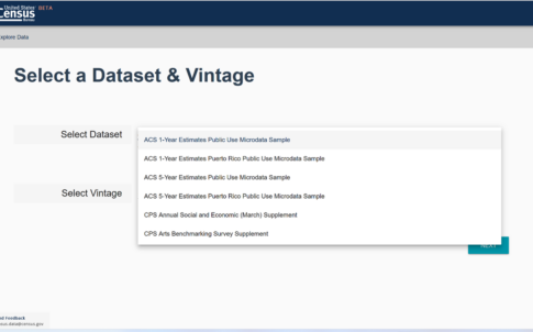
On the MDAT website, we need to select a dataset and a vintage (year).
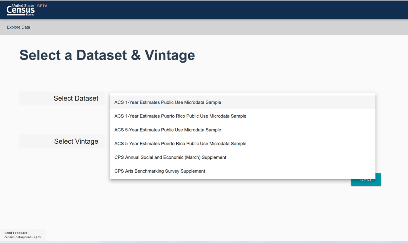
First, we need to know whether the data appears in the American Community Survey or the Current Population Survey. We can check the subject tables for the American Community Survey (ACS) and the Current Population Survey and see that marital history and status is in the ACS. On the landing page of MDAT we choose our survey and our “vintage” (year).
Next, we select the variables we need. In our example we need a variable for race/ethnicity and one for married in the last 12 months. Before we begin looking for our variables it can be helpful to look through the data dictionary for the American Community Survey (the Current Population Survey consists of the monthly surveys and two supplemental surveys: the Annual Social and Economic Supplement (ASEC) and the annual fertility supplement). Note that the variables can change between years. There are three ways to find our variables in the MDAT tool.
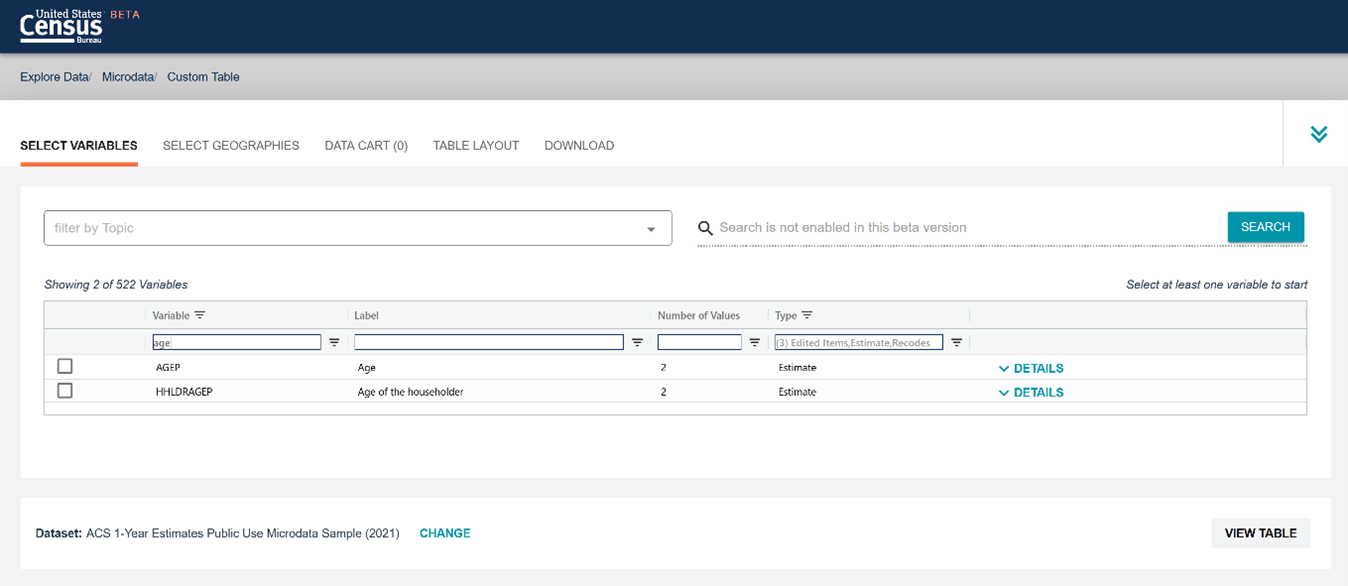
1. If we already know the variable name we can type it into the search bar under “Variables.” Some variables e.g. demographic variables such as sex and age are easier to find.
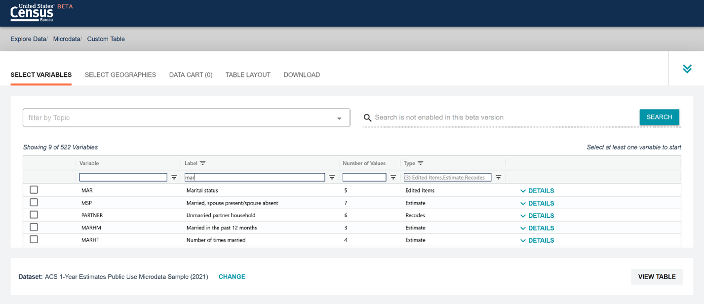
2. We can search for the name of the variable in the search bar under “Label.” The variables might have very specific labels. For instance, if we type “married” in the search bar we can find married within the last 12 months but if we type “marry” it will not show up.
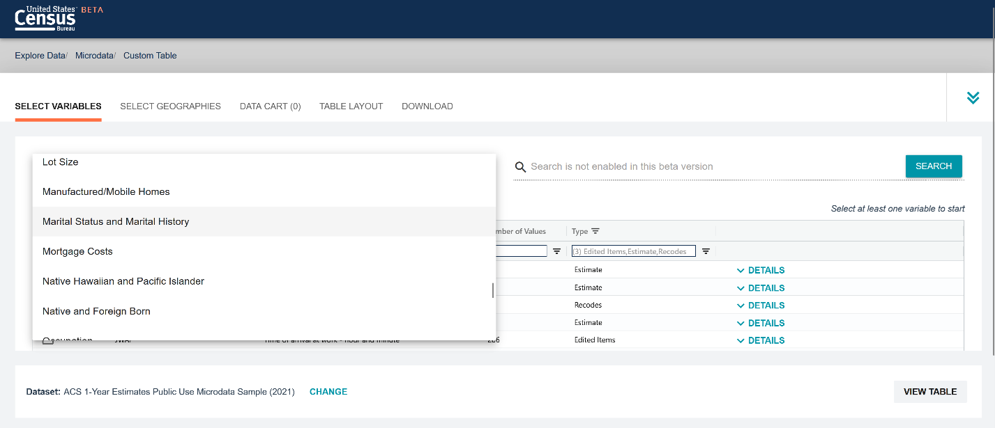
3. The last way to find the variables we need is to filter by topic. To find the variable for married within the last 12 months we would select “Marital Status and Marital History.”
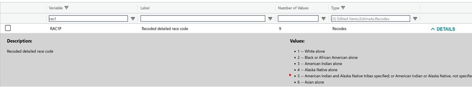
To select a variable for race and any additional variables we would go through the same steps. We can click on details to see more information about the variable, for instance what racial/ethnic groups are included in the race variable.
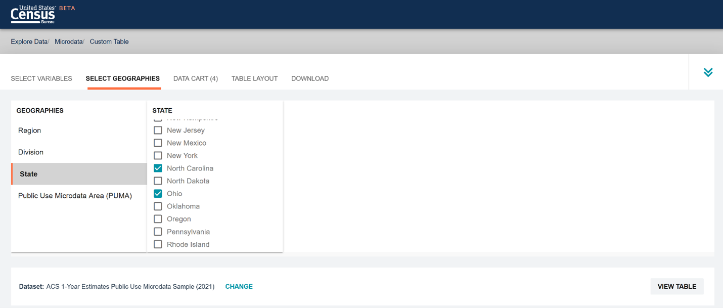
When we have selected all the variables we need we go to the geographies tab to select our level of geography or area of interest. We can further narrow down our example and look at North Carolina and compare it to other states. To do so we choose State and North Carolina from the drop-down menu. A drawback of this feature is that if we wanted to look at how North Carolina compares to all 50 states we would need to select each state individually. For this example, we can choose Ohio as a comparison state (they are of similar population size).
Next we go to our data cart where we can see what variables we have selected and information about them. We can also create new variables if needed by recoding an existing variable.
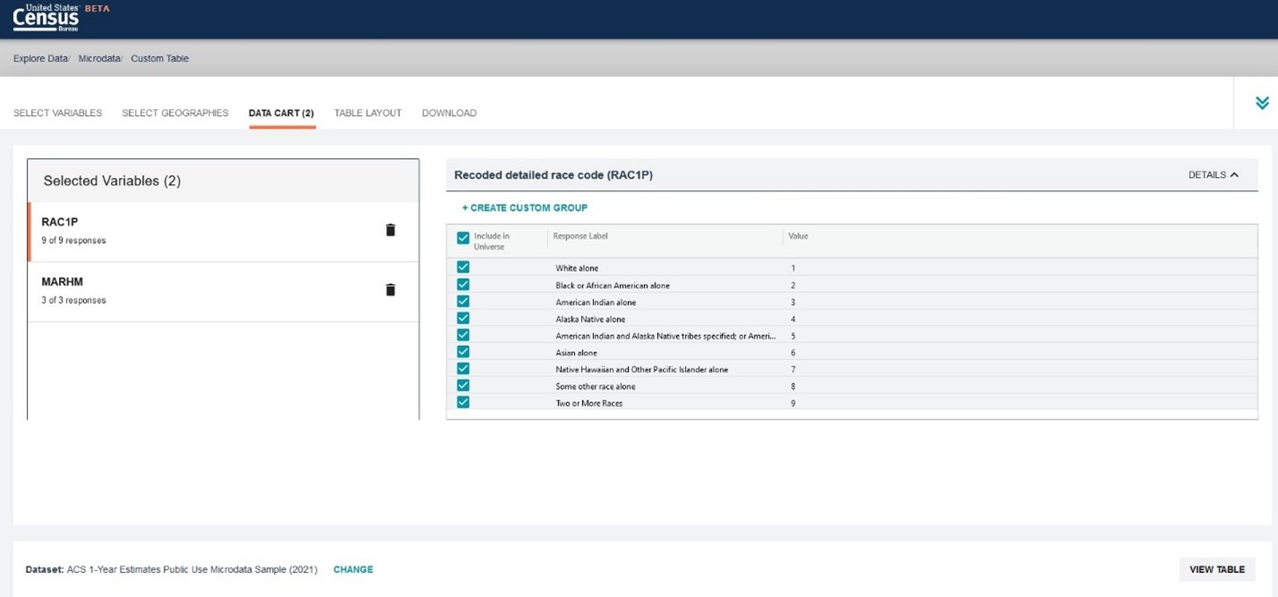
Here we can create a new race variable and to simplify the example we only compare Black and White individuals. To create a new variable, we choose only the groups “Black or African American alone” and “White alone” and click “create custom group.”
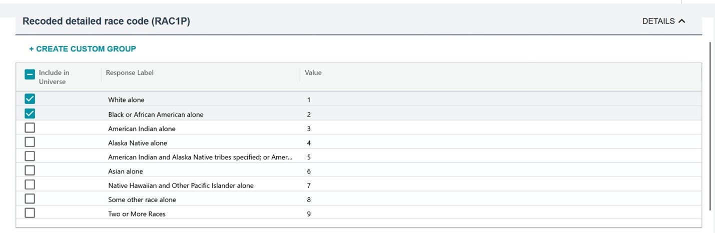
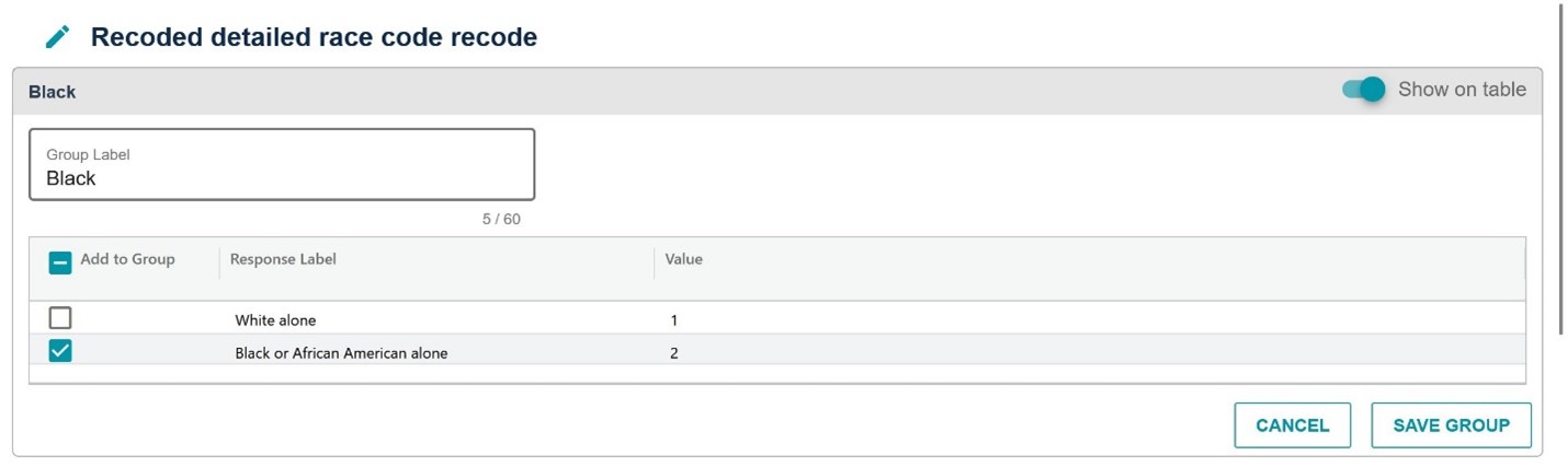
We can rename this group “Race” and save the variable. We now have a variable called “RAC1P_RC_1” (RC stands for “recode.”) We then need to create one group for the White population and one for the Black population. We create the groups one at a time and save each group. First we create a group called Black and only select Black or African American alone and save this group.
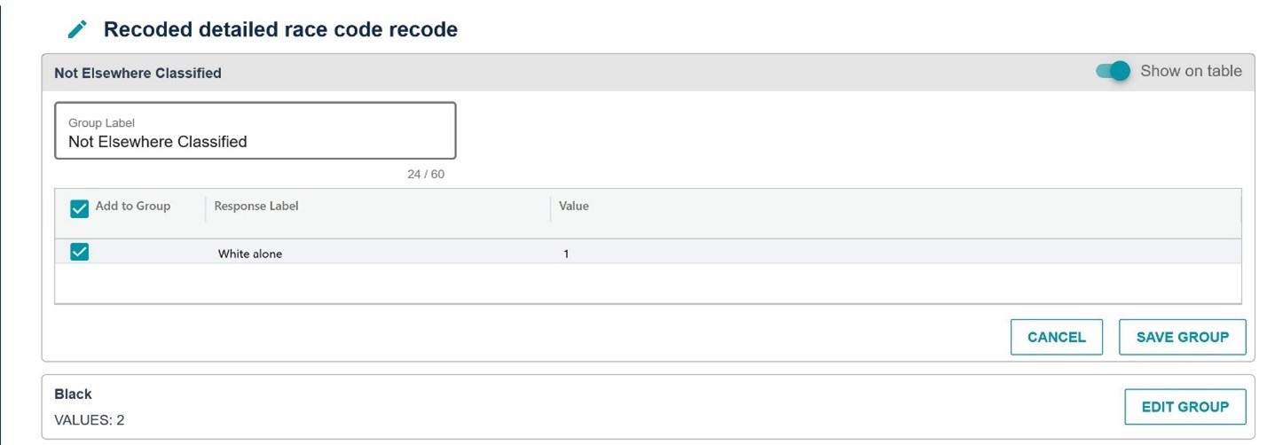
Next we create the group for White by clicking the “Not Elsewhere Classified” category, select White alone, rename the label, and save the group. We now have a variable for race that is limited to the Black and the White populations. If we wanted to keep all other races/ethnicities but not display them on the table, we could code a third group (don’t unselect any categories when clicking create custom group) and unselect “show on table” for the third group.
If we want to work with continuous variables such as age they need to be recoded as groups. For the example we can create an age variable that will limit the sample to those ages 15 to 50. The steps are similar to how we created the new race variable, but instead of selecting a group we need to create ranges of years.
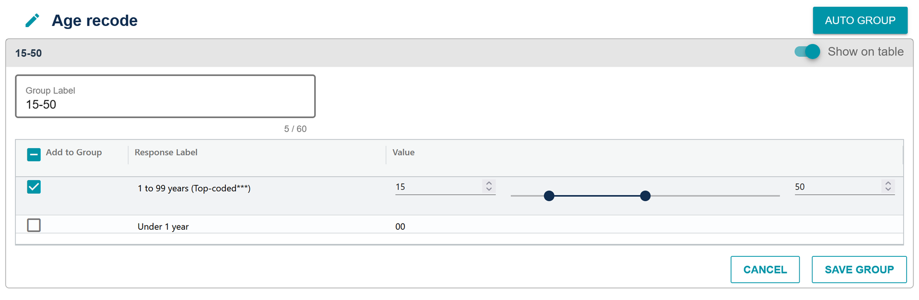
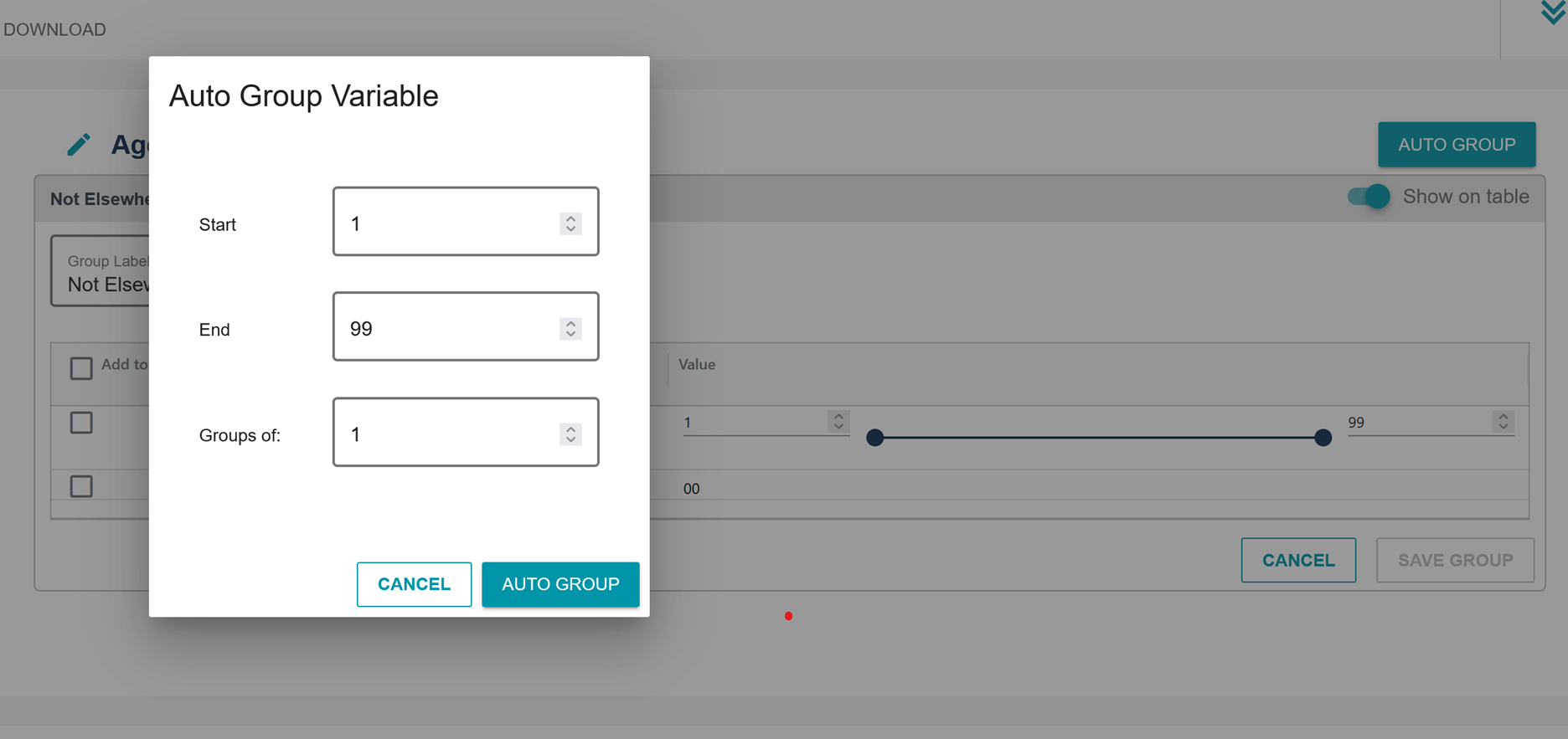
If we wanted to look at something by age and use all ages we can instead of creating one group for each year of age at a time use the “auto group” option. We can choose the youngest and the oldest ages we want to look at and the interval between the years. Other continuous variables such as income work in the same way. We can choose any size group we want, e.g. single year, five year intervals etc.
Next we can look at our table and change the layout to how we want it look. If we go to Table Layout we can see how the table currently looks. We can change up the rows and the columns to any way we want, the tabulations will be the same regardless of where a variable is placed. MDAT does not include any numbers during the table layout stage so that the table will load quicker.
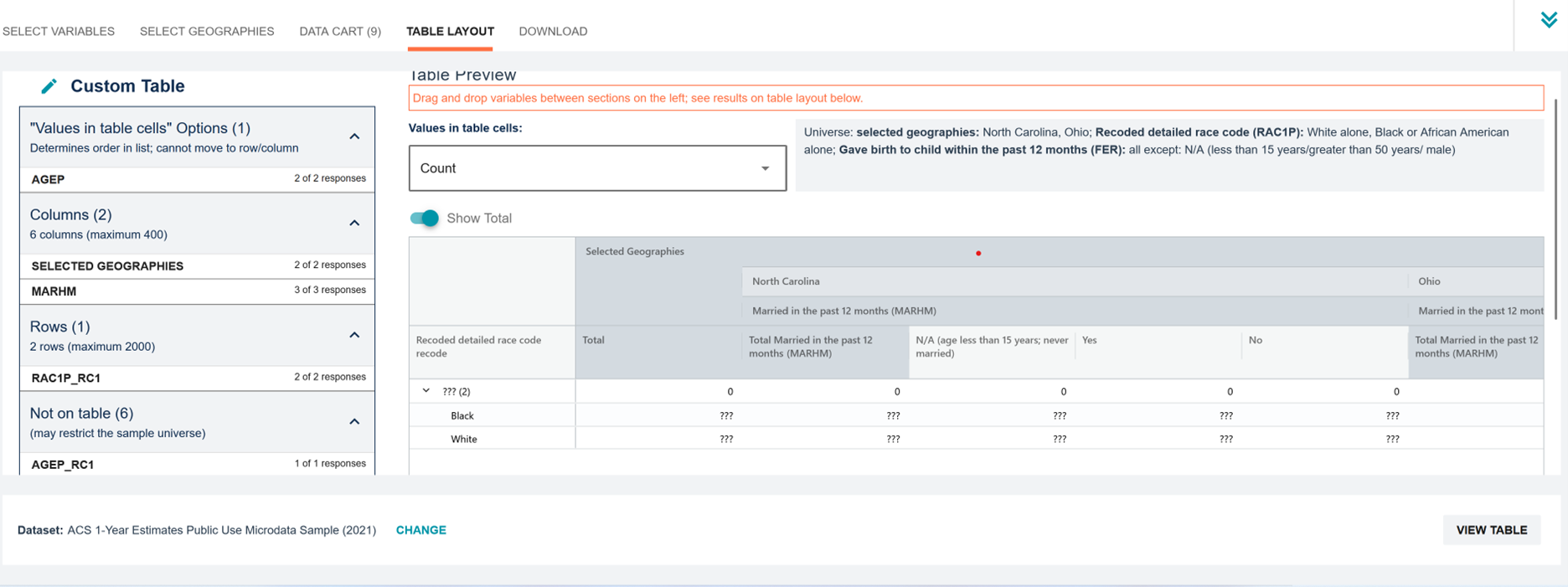
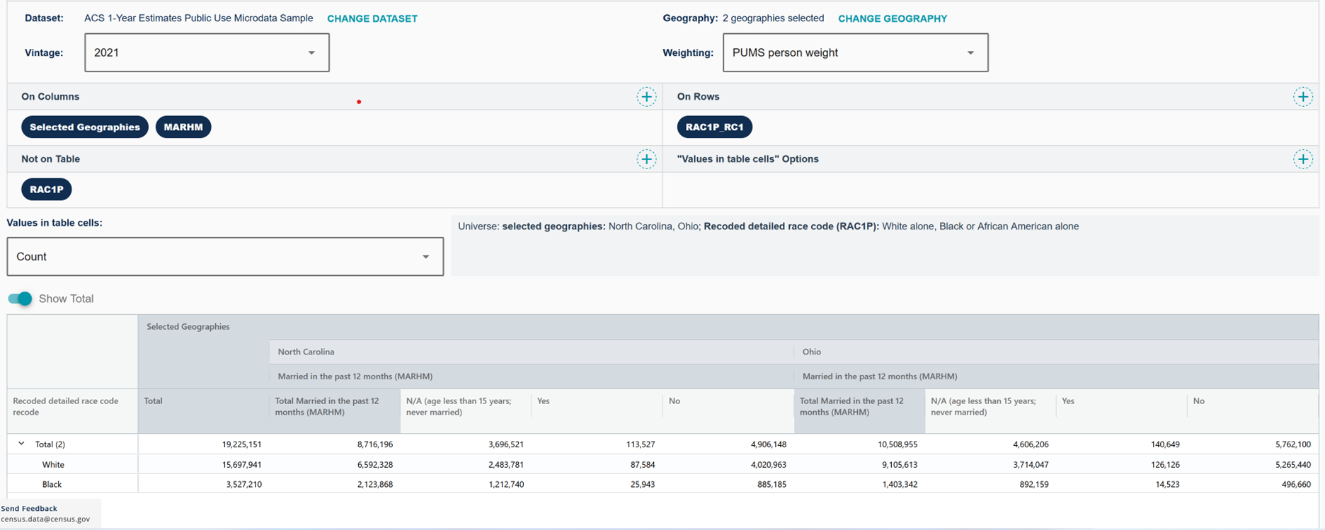
To change the layout, click and drag the variables to the row or column section. To remove a variable from the table drag it to the bottom section (note that these variables might still be limiting the sample to a specific group.) After rearranging the variables, the table now shows race in the rows and geographies and married in the last 12 months in the columns. The order of the variables in the columns and rows also matter: the variables are nested within each other, e.g. married in the last 12 months is nested within each state in our example.
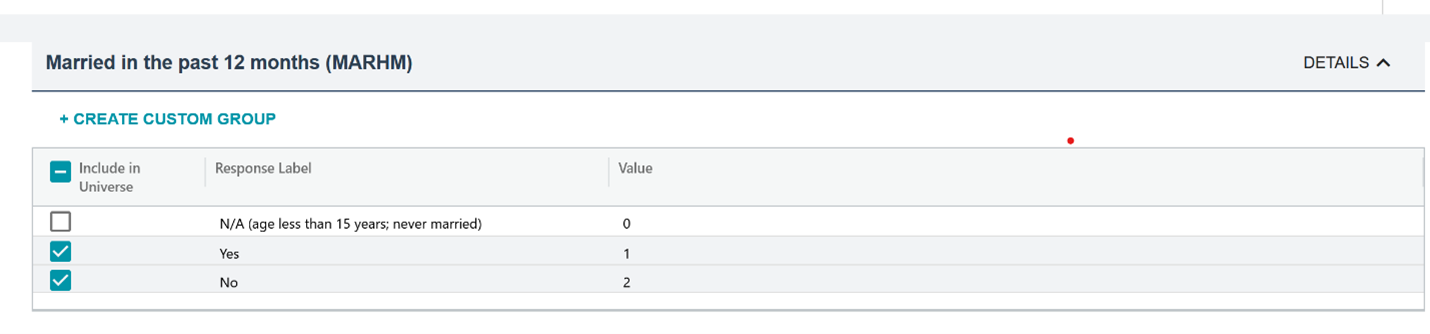
For married in the last 12 months there is an additional category to yes and no – those who are under 15 or never married and not applicable in the measure. If we go back to the data cart we can select that variable and unselect the N/A category so that it does not show on the table.
When the table looks like we want it we can click “view table.” Here we will get the real numbers. Disclaimer: if the data set we are using is big, the loading time can be long. At this stage it is still possible to rearrange the table by clicking and dragging a variable from e.g. row to column.
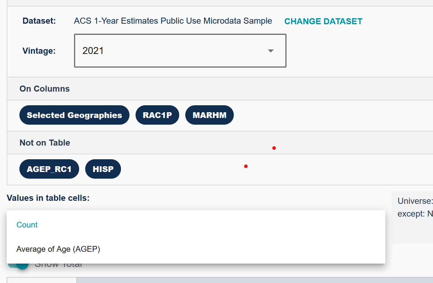
If no numbers show up, check that “count” is selected and not “average of age” (unless mean age is what is of interest.)
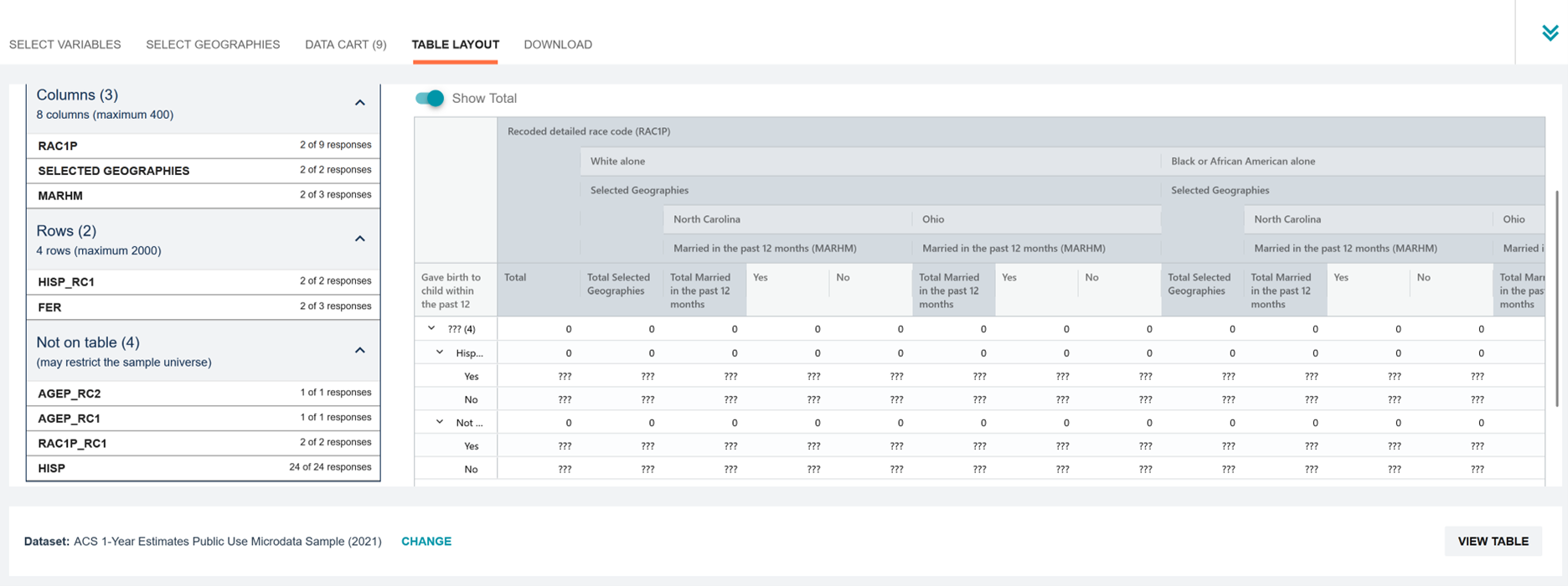
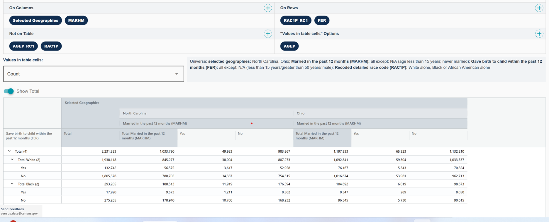
We can also look at a topic in even more detail than above. Say that we want to know the estimated number of women who both married and had a child in the last 12 months by race/ethnicity. We can add the variable for having a child in the last 12 months by clicking any of the + signs on the rows and columns or click “customize variables” and go back to the data cart (clicking on a variable also takes us back to the data cart and we can also recode these variables again). It does not matter if we add a variable to the rows, columns, or not on table as we can move it at a later time. We can then arrange the table to best show the data. The new more specific estimates are in the table below.
Lastly, there are several ways to download the data.
First, we can choose to download the table as it currently looks. This gives us a table like the one below.
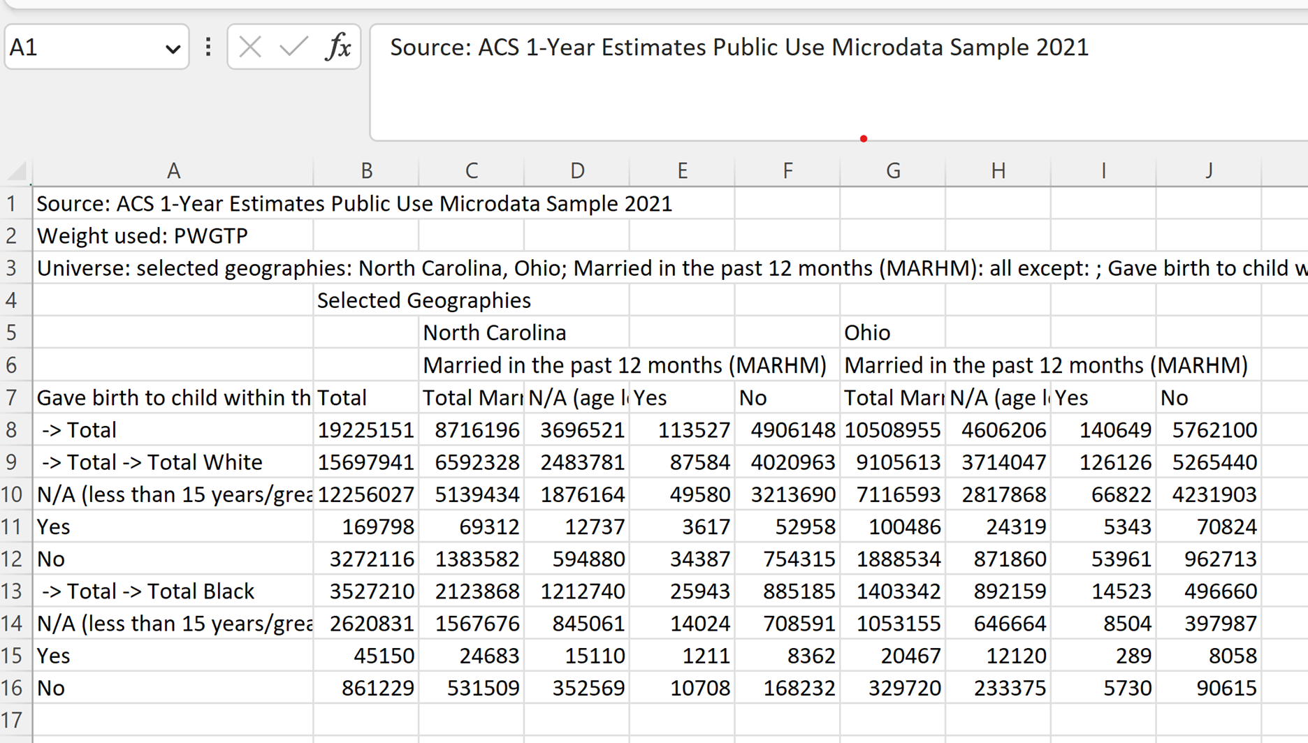
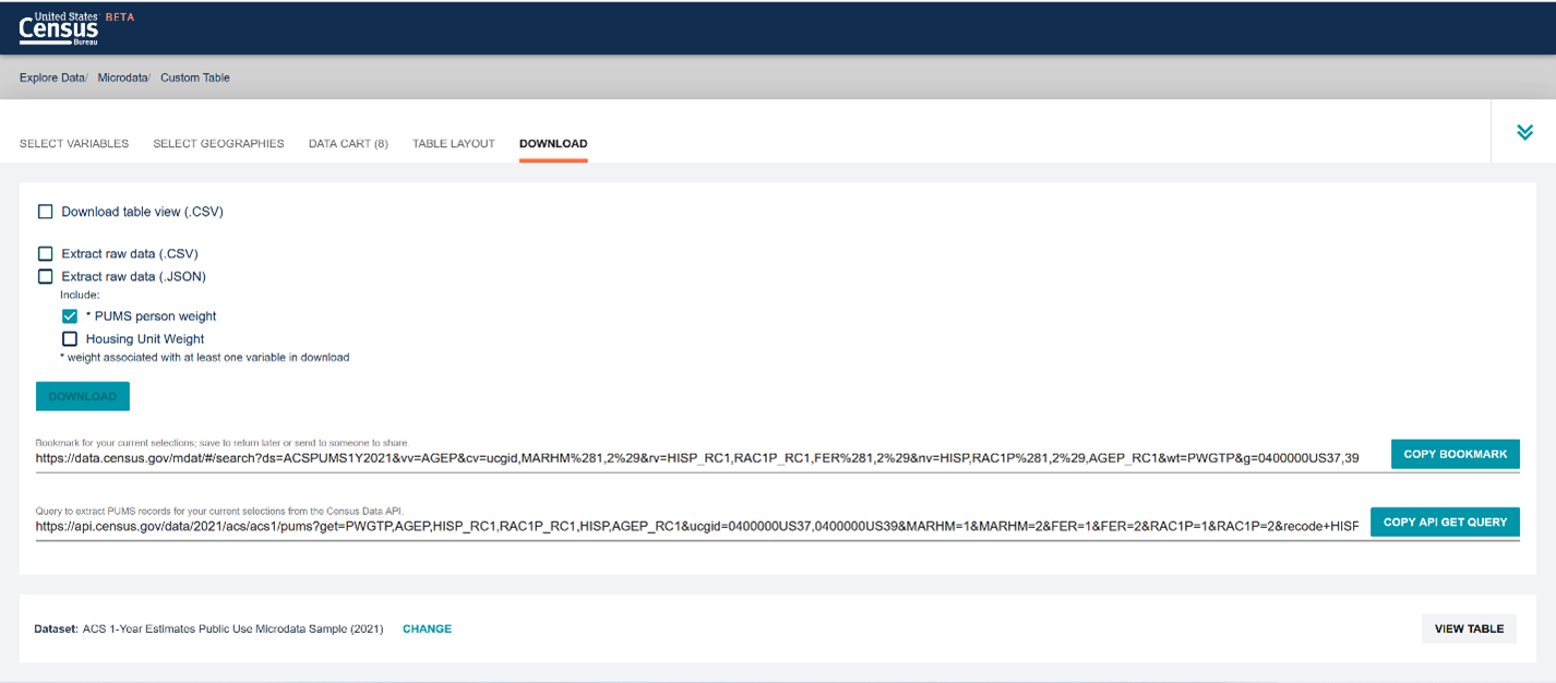
Second, we can download microdata to use in statistical software. If we are more interested in choosing variables to download to use with statistical software, we can skip the table stages and just add the variables we need and download the csv file. The person weights are added to the data by default but we need to add any identifier such as the serial number (called serialno in the data) for the household serial numbers and select the household weight (if needed) ourselves if we are working with household level data.
Third, in the download tab we can also choose to download our data using API. We can download the data as microdata “copy API get query” or as a table “copy API tabulate query.” We can also bookmark the page and go back to our customized table at any time or share the table with others.
ACS subjects https://www.census.gov/programs-surveys/acs/guidance/subjects.html
CPS subjects https://www.bls.gov/cps/cps_over.htm#available
Need help understanding population change and its impacts on your community or business? Carolina Demography offers demographic research tailored to your needs.
Contact us today for a free initial consultation.
Contact UsCategories: Story Recipe

The Center for Women’s Health Research (CWHR) at the University of North Carolina School of Medicine released the 12th edition of our North Carolina Women’s Health Report Card on May 9, 2022. This document is a progress report on the…

Dr. Krista Perreira is a health economist who studies disparities in health, education, and economic well-being. In collaboration with the Urban Institute, she recently co-led a study funded by the Kate B. Reynolds Foundation to study barriers to access to…

Our material helped the NC Local News Lab Fund better understand and then prioritize their funding to better serve existing and future grant recipients in North Carolina. The North Carolina Local News Lab Fund was established in 2017 to strengthen…
Your support is critical to our mission of measuring, understanding, and predicting population change and its impact. Donate to Carolina Demography today.